|
Tsunami Source Models of the 2011 Off the Pacific Coast of Tohoku Earthquake
(Ver. 6.2, Ver. 7.0 and Ver. 8.0)
|
We performed multiple time-window tsunami waveform inversions to estimate the temporal and spatial distribution of fault slips of the Tohoku earthquake (38.322°N, 142.369°E, Mw = 9.0 at 5:46:23 UTC according to USGS) on March 11, 2011. We assumed 44 or 55 subfaults which are located within the aftershock area (Fig. 1). A rupture velocity of 2.0 km/s was assumed from the epicenter to an edge of each subfault.
Ver. 6.2: 44-subfault model. The length and width are 50 km × 50 km for each subfault. The focal mechanisms of the all subfaults are strike:193º, dip:14º and slip:81º from the USGS's Wphase moment tensor solution. The top depths of the subfaults were assumed to 0 km, 12.1 km, 24.2 km and 36.3 km for near-trench, shalow, middle and deep subfaults, respectively.
Ver. 7.0 [Satake et al., 2013]: 44-subfault model. The length and width are 50 km × 50 km for each subfault. The strike and slip angles are 193º and 81º, respectively, from the USGS's Wphase moment tensor solution. The dip angles are assumed from the plate boundary model [Nakajima and Hasegawa, 2006]. They are 8º, 10º, 12º and 16º from near-trench to deep subfaults. The top depths of the subfaults were assumed to 0 km, 7.0 km, 15.6 km and 26.0 km for near-trench, shalow, middle and deep subfaults, respectively.
Ver. 8.0 [Satake et al., 2013]: 55-subfault model. The near-trench subfaults are halved for the width (i.e. 25 km) from Ver. 7.0. The other fault parameters are the same with Ver. 7.0. The top depths of the subfaults were assumed to 0 km, 3.5 km, 7.0 km, 15.6 km and 26.0 km from near-trench to deep subfaults.
Fault parameters are here (Ver. 6.2) and (Ver. 7.0) and (Ver. 8.0)
Snapshots of temporal slips on the faults are here (Ver. 6.2) and (Ver. 7.0) and (Ver. 8.0)
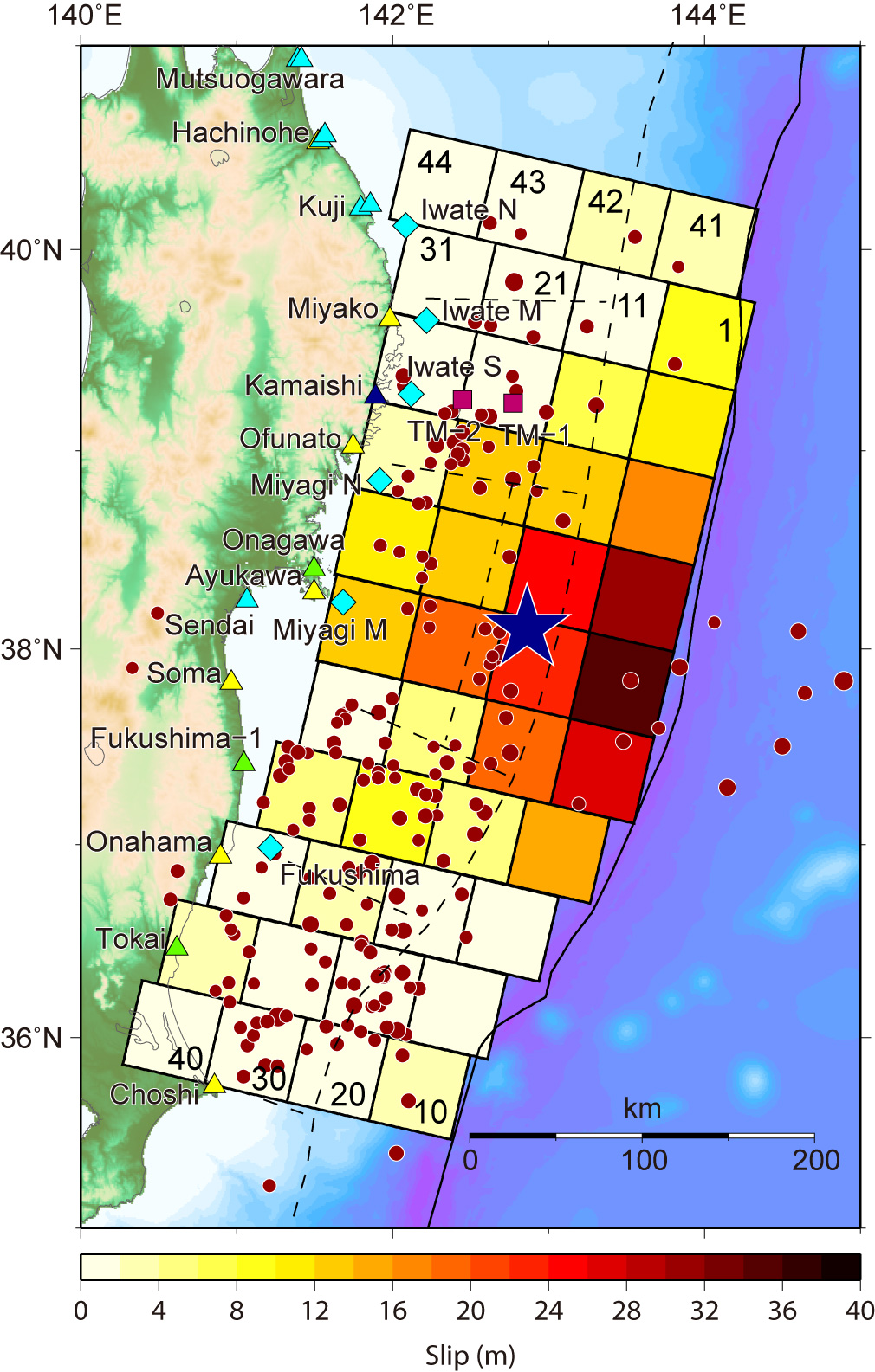
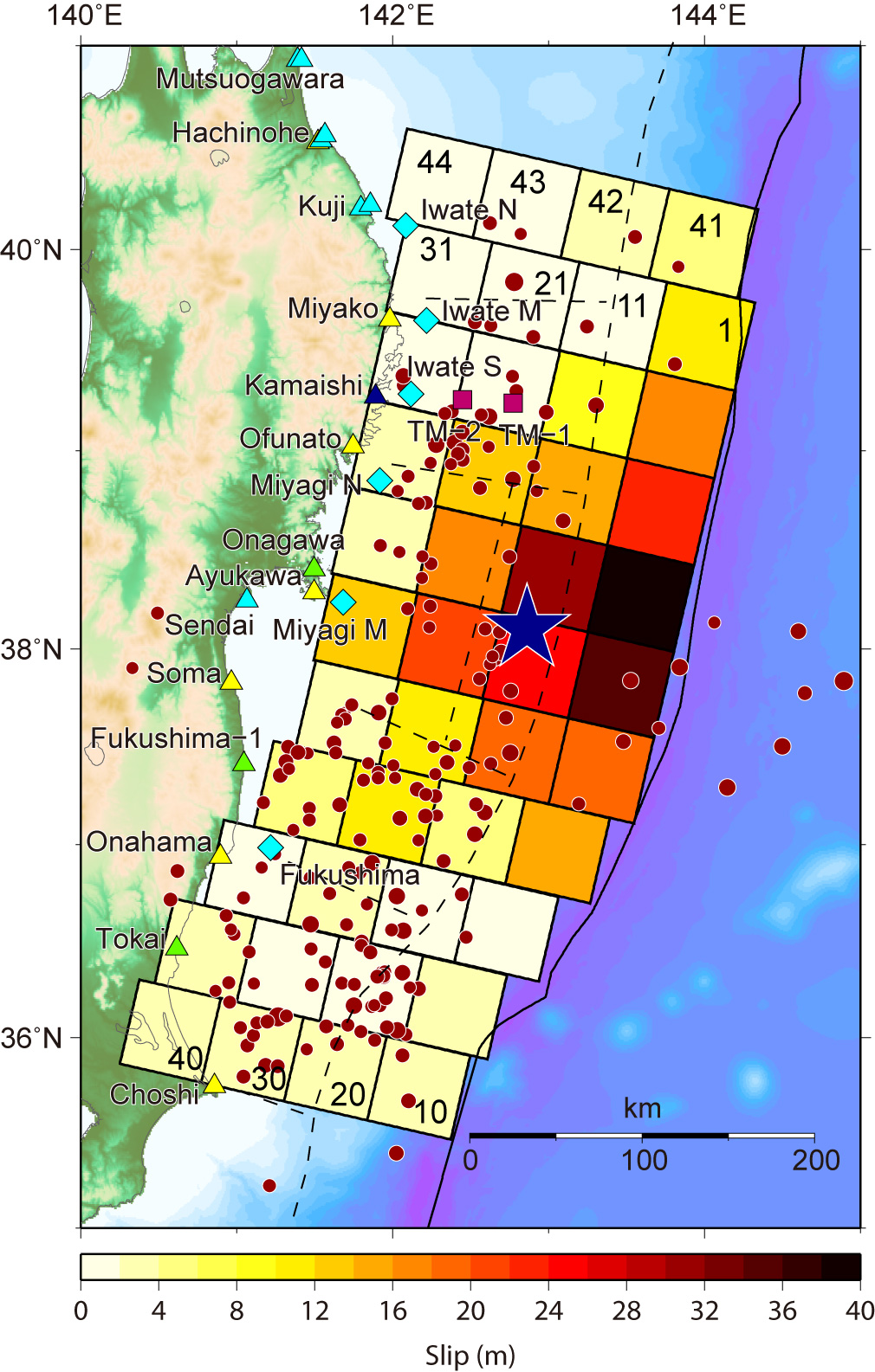
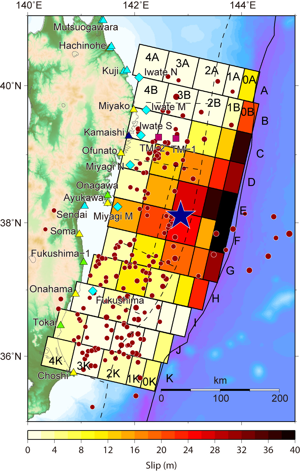
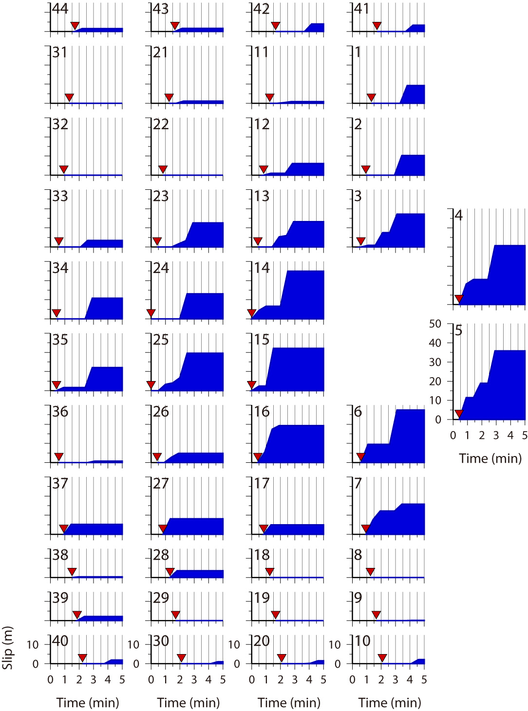
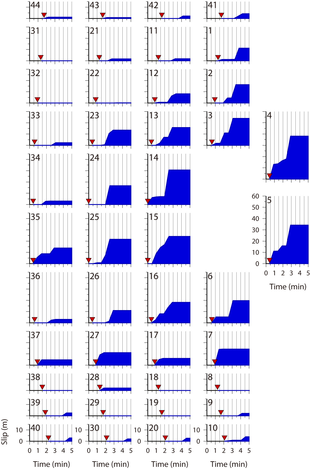
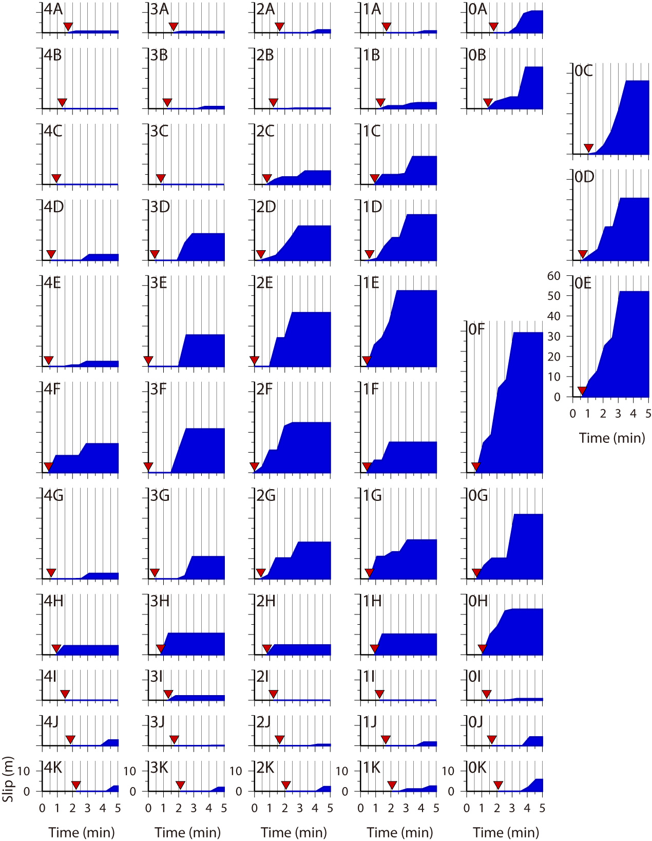
Fig.1 Tsunami Source Models, Left: Ver. 6.2, Middle: Ver. 7.0, Right: Ver. 8.0
Upper: Slip distribution on the fault model. Mainshock (Blue star) and aftershocks (determined by JMA) during about one day after the mainshock are also shown by red circles.
Lower: Spatial and temporal distribution of slip on subfaults. Temporal changes of slip after the rupture onset (inverse triangles, assuming a rupture velocity of 2.0 km/s) with 30 s interval are estimated.
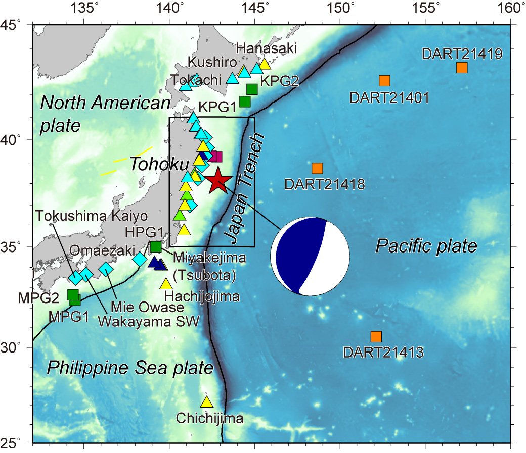
Fig.2 Offshore stations, tide and wave gauges used for the inversion.
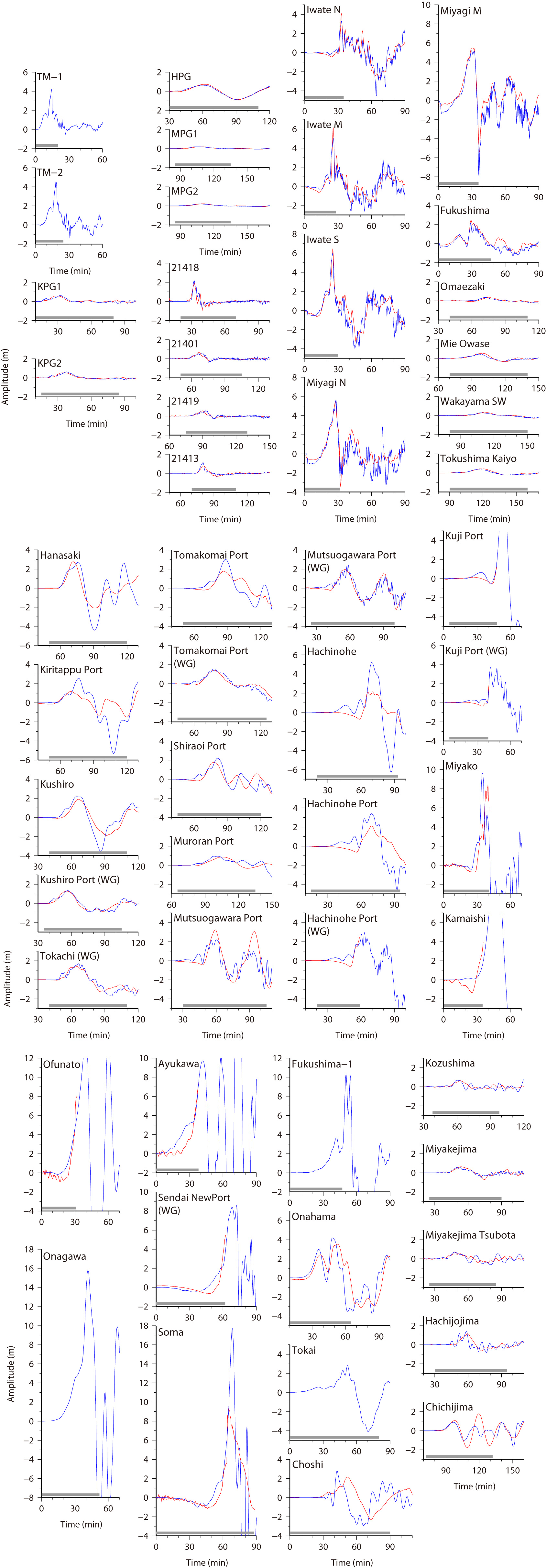
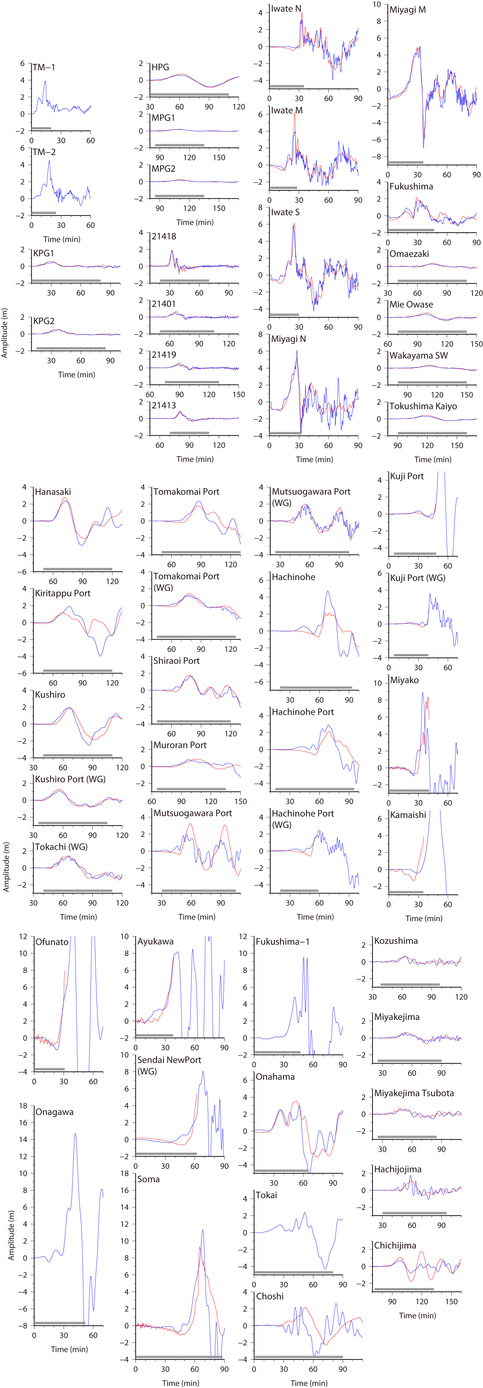
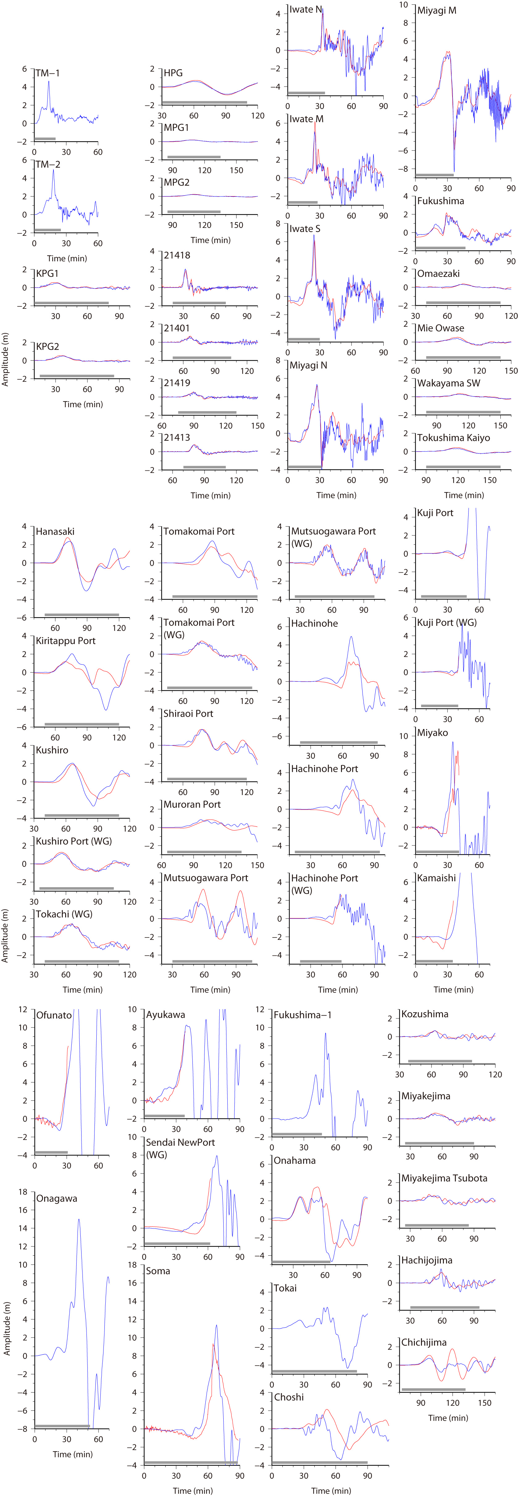
Fig.3 Simulated Tsunami around Japanese coasts, Left: Ver. 6.2, Middle: Ver. 7.0, Right: Ver. 8.0
Red and blue lines indicate the observed tsunami waveforms and synthetic ones, respectively. Gray bars show the time windows used for inversion.
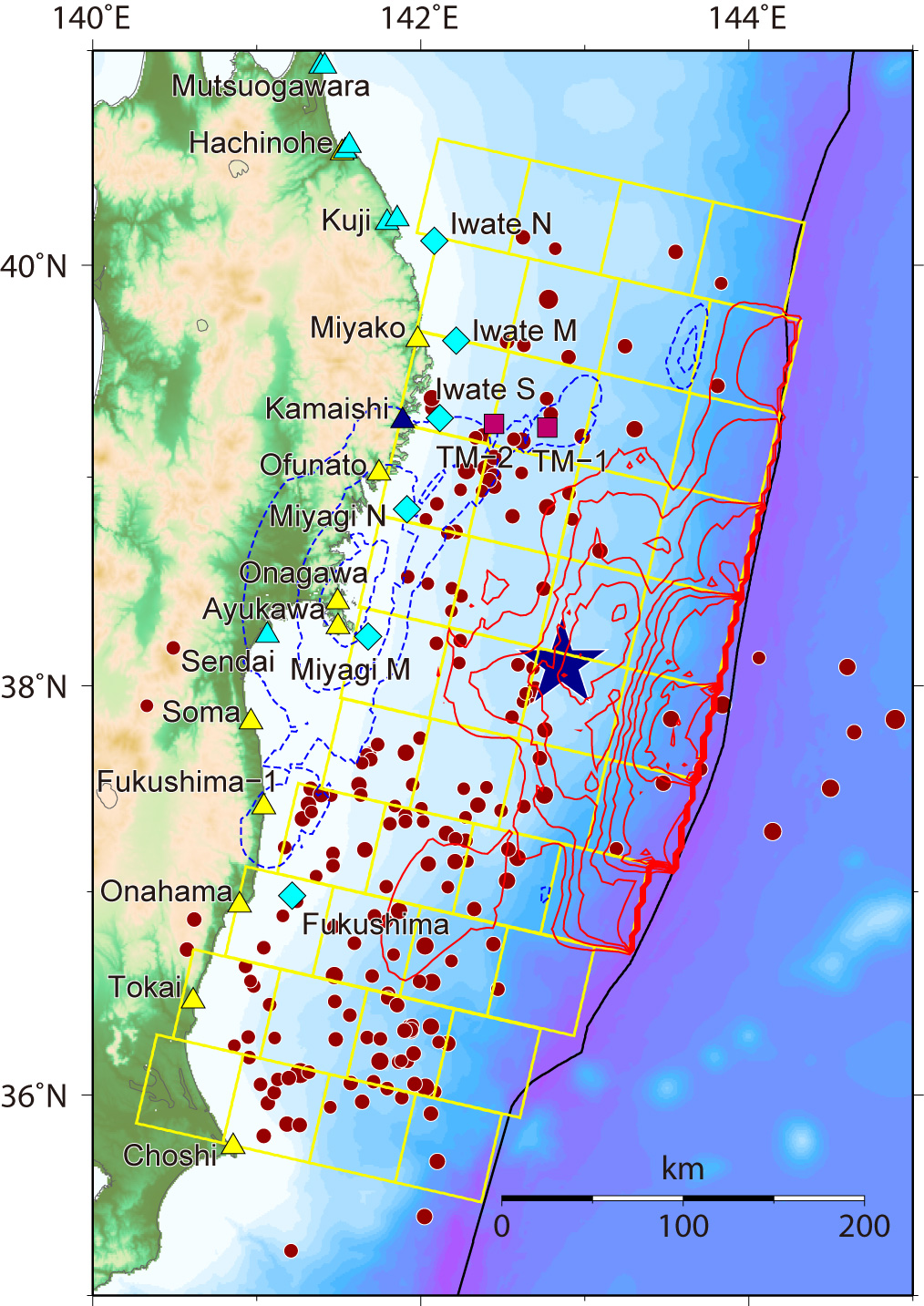
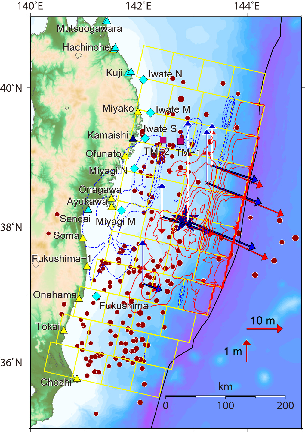
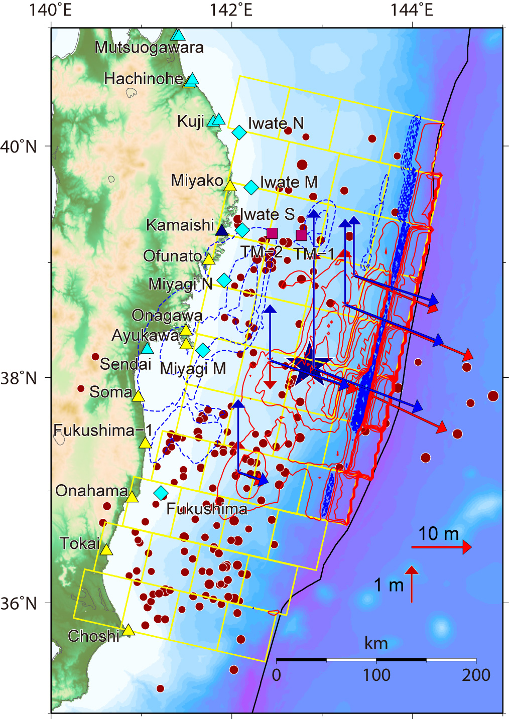
Fig.4 Seafloor Deformation, Left: Ver. 6.2, Middle: Ver. 7.0, Right: Ver. 8.0
Calculated seafloor deformation due to the fault model. The red contours indicate uplift with the contour interval of 1.0 m, while the blue contours indicate subsidence with the contour interval of 0.5 m.
Observed displacements by the GPS/A measurements [Sato et al., 2011] are compared with the predicted displacements by the inversion models.
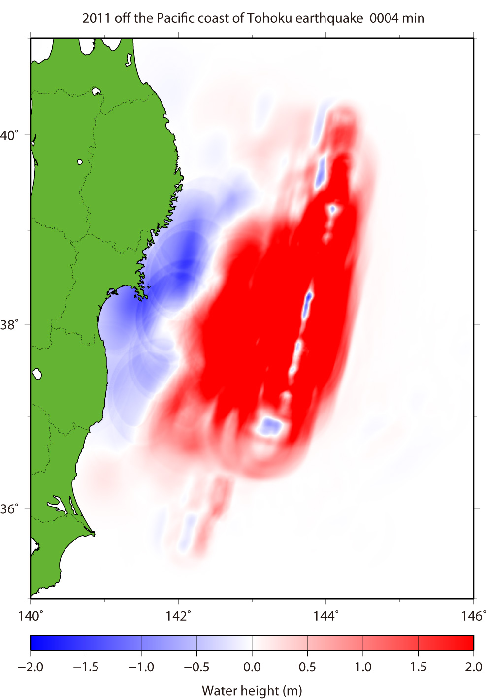
Fig.5 Tsunami Propagation (Click to start animation) for Ver. 8.0
The red color means that the water surface is higher than normal sea level, while the blue means lower.
| by Yushiro Fujii (IISEE, BRI) and Kenji Satake (ERI, Univ. of Tokyo) |
|
|
| References |
|
Nakajima, J. and Hasegawa, A. (2006). Anomalous low-velocity zone and linear alignment of seismicity along it in the subducted Pacific slab beneath Kanto, Japan: Reactivation of subducted fracture zone? Geophys. Res. Lett., 33, L16309, doi:10.1029/2006GL026773 Okada, Y. (1985), Surface Deformation Due to Shear and Tensile Faults in a Half-Space, Bull. Seismol. Soc. Am., 75, 1135-1154. Satake, K. (1995), Linear and Nonlinear Computations of the 1992 Nicaragua Earthquake Tsunami, Pure and Appl. Geophys., 144, 455-470. Satake, K., Fujii, Y., Harada, T. and Namegaya Y. (2013),Time and Space Distribution of Coseismic Slip of the 2011 Tohoku Earthquake as Inferred from Tsunami Waveform Data, Bull. Seismol. Soc. Am., accepted. Sato, M., Ishikawa, T., Ujihara, N., Yoshida, S., Fujita, M., Mochizuki, M. and Asada, A. (2011). Displacement above the hypocenter of the 2011 Tohoku-Oki earthquake. Science, 332(6036), 1395-1395. |
Last Updated on 2012/8/17